
Shape Regularization
Published:
Shape Regularization
Nail Ibrahimli, Shenglan Du
1 Background
We live in a 3 Dimensional (3D) world that is composed of urban entities such as buildings and streets. In recent years, there is an ever-increasing demand, both by academia and industry, for 3D spatial information and 3D city models [Biljecki et al., 2015]. Modelling urban scenes from 3D data has become a fundamental task for various applications such as architecture design, infrastructure planning, land administration, and city management.
One common way to obtain 3D models of buildings is to reconstruct the surface meshes from point clouds (i.e., a discrete data representation of the surrounding space acquired from LiDAR systems). There exist amounts of works for point cloud reconstruction [Kazhdan et al., 2006; Nan and Wonka, 2017]. Although point clouds can well preserve the raw geometric information of the urban objects, the reconstructed models still suffer from issues such as data noises and undesired structures. The goal of this assignment is to:
- Optimize the model geometry with the minimum refinement effort.
2 Dataset Explanation
Given a noisy reconstructed polyhedron mesh model with N vertices, we want to find the minimum change of the coordinates to make the model geometry regular. Figure 1 gives a visualization of the 4 models which we use to test our algorithm.
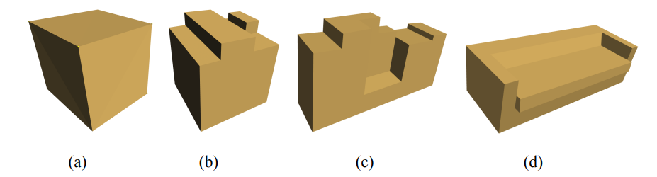
Figure 1. Visualization of the input models.
3 Problem Statement
We directly take the points P of the polyhedron model as input to our optimization algorithm, which could be formulated as
\[P=(x_1, y_1, z_1, x_2, y_2, z_2, x_3, y_3, z_3, ... , x_n, y_n, z_n)\]where each $(x,y,z)$ represents the 3D coordinates of a point of the model, n represents the total number of points of the model. Clearly, we have $P \in R^{3n}$.
As the model is noisy, its geometry is usually not perfectly regular. For instance, pair edges/faces which suppose to be parallel are not perfectly parallel, and intersected edges/faces which suppose to be orthogonal are not perfectly orthogonal (Figure 1 gives a visualization of the noisy models with irregular geometry).
In this project, we aim to find the minimum change of the coordinates $\Delta P$ to make the model geometry regular. we focus on one specific geometrical constraint:
- near-orthogonal edges should be perfectly orthogonal.
3.1 Data preprocessing
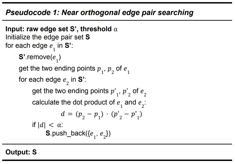
We start by searching for near-orthogonal pairs of edges of the model. These edge pairs will form the orthogonal constraints later. The main idea is to loop over all possible combinations of edges in the model, calculate their intersecting angles, and if the angle is near 90 degrees, then store the corresponding edge pair in a set S.
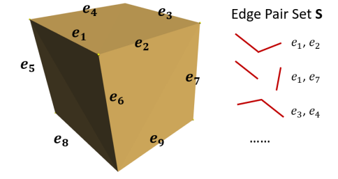
Figure 2. Near-orthogonal edge pairs of a cube model.
3.2 Problem Formulation
Our goal is to find a new vector $X \in R^{3n}$ which produces perfect orthogonal relationships for all the edge pairs in the set S (S has been obtained from the preprocessing step), and at the meantime, generates the least cost of modifying the model geometry $||X-P||_2$ .
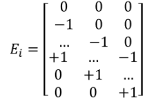
Assume we have an edge $e_i$ with a starting point $p_s$ and a tail point $p_t$, the geometry of $e_i$ can be represented as:
\[(x_t-x_s,y_t-y_s,z_t-z_s)\]In a matrix formulation the geometry should be:
\[X^TE_i\]where $E_i$ is a $3n \times 3$ matrix. The elements of $E_{(3s,0)},E_{(3s+1,1)}$ and $E_{(3s+2,2)}$ are -1, while the elements of $E_{(3t,0)},E_{(3t+1,1)}$ and $E_{(3t+2,2)}$ are +1. All the rest elements are 0.
Similarly, for another edge $e_j$, we can represent its geometry as: \(X^TE_j\) Given an edge pair {$e_i,e_j$} in the set S, we exploit their orthogonal relationship by calculating the dot product of the two edge vectors:
\[d = (X^TE_i) \cdot (X^TE_j) = X^TE_i(X^TE_j)^T= X^TE_iE_j^TX\]
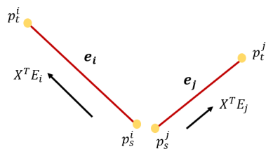
Figure 3. Visualization of an edge pair
Therefore, the problem is formulated as
\[\text{ min } ||X-P||_2 \\ s.t.\ X^TE_iE_j^TX = 0, \text{ and } (i,j) \in S\]where $X\in R^{3n}$ is the variable we want to optimize over. $P\in R^{3n}$ is the vector of the raw point 3D coordinates. $S$ is the set of near orthogonal edge pairs that is obtained during the Section 3.1 data preprocessing step.
3.3 Problem Approximation
In Section 3.2 we give the true formulation of the problem, which has a convex objective function and several quadratic equality constraints. Obviously, it is not a convex problem.
For solving the problem with a gradient-based method, we approximate this non-convex problem into a convex problem. Inspired by the strategy of weight regularization which is commonly used in deep learning neural networks [Goodfellow et al., 2016], we transfer the quadratic constraints as a regularization term of the existing objective function.
The approximate optimization is formulated as
\[\text{min } ||X-P||_2 + \lambda \sum_{i,j\in S} |X^TE_iE_j^TX|\]where $\lambda$ is a constant term that determines how much influence the orthogonal regularizer contributes to the objective function. $ |\cdot | $ gives the absolute value of the term inside.
In this way, we eliminate the quadratic constraints and approximate the problem to an unconstrained convex problem. We can easily solve this problem using the gradient descent method. More specifically, we refer to a sub-gradient method, as the absolute function $ |\cdot | $ doesn’t have its gradient when the inside term reaches 0. Section 4.2 gives a detailed derivation of the gradient method and our experimental parameters of $\lambda$ and learning rate $\eta$.
4 Implementation Details
We implemented both optimizers in Modern C++ (versions after >= C++11). We have used Easy3D [Nan, 2021] for linear algebra operations and for rendering. The source code and the datasets are available at:
https://github.com/Mirmix/3D_shape_regularization
4.2 Solving with the Sub-Gradient Method
We have used the Eigen library for Linear Algebra operations. According to Section 3.3, we have derived our loss function as follows. Our goal is to minimize this loss function using the sub-gradient descent method.
\[\mathcal{L} = ||X-P||_2 + \lambda \sum_{i,j\in S} |X^TE_iE_j^TX|\]The total loss is composed of two parts. The first term penalizes based on the L2 norm of $X$ deviation from input $P$. The second L1 norm functions as an orthogonal regularizer, which penalizes over the residual of the inner product of two orthogonal edges.
The gradient of the first term w.r.t $X$ is $2(X-P)$, while the second term is more tricky, because it depends on the sign of each term $ |X^TE_iE_j^TX| $ for all edge pairs {$i,j$} in the set S. According to that, we give the pseudocode of the sub-gradient descent method:
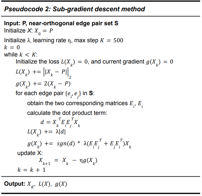
While updating the gradient $g(X_k)$, we decide to choose plus or minus based on the sign of each single dot product term $X_k^TE_iE_j^TX_k$. Thus, $X_{k+1} = X_k-\eta g(X_k)$ helps us iteratively approach to optimal solution via gradient scaled by the learning rate. Additionally, we have 2 hyperparameters to be tuned: $\lambda$ and $\eta$.
We have experimented with our sub-gradient descent method over the 4 models. Figure 4 gives the visualization of the losses during the optimization process. Different colours indicate the loss convergence for different models. The legend on the top right describes the model names. The visualization shows that our algorithm is effective for all the input models.
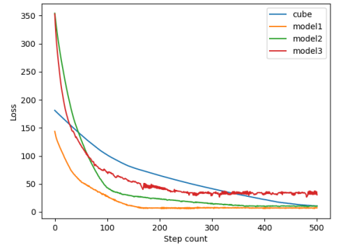
Figure 4. Loss convergence of the 4 models over 500 steps
References:
[1] Biljecki, F., Stoter, J., Ledoux, H., Zlatanova, S., and Coltekin, A. (2015). Applications of 3d city models: State of the art review. ISPRS International Journal of Geo-Information, 4(4):2842-2889.
[2] Goodfellow, I., Bengio, Y., & Courville, A. (2016). Deep learning. MIT press.
[3] Kazhdan, Michael, Matthew Bolitho, and Hugues Hoppe. “Poisson surface reconstruction.” Proceedings of the fourth Eurographics symposium on Geometry processing. Vol. 7. 2006.
[4] Nan, L., & Wonka, P. (2017). Polyfit: Polygonal surface reconstruction from point clouds. In Proceedings of the IEEE International Conference on Computer Vision (pp. 2353-2361).
[5] Nan, L. (2021). Easy3D: a lightweight, easy-to-use, and efficient C++ library for processing and rendering 3D data.