Multi-view stereo (MVS) is a computer vision technique for reconstructing a 3D model of a scene from a set of 2D images taken from different calibrated views. It is an important problem in computer vision and has many applications, including robotics, virtual reality, and cultural heritage preservation.

The goal of MVS is to recover the 3D structure of a scene from a set of images taken from different viewpoints. This is typically done by finding correspondences between points in the different images and using them to triangulate the 3D positions of the points. Once the 3D positions of the points are known, they can be used to generate a 3D model of the scene.

MVS algorithms can be divided into two main categories: dense MVS and sparse MVS.

• Dense MVS algorithms aim to reconstruct a dense 3D model of the scene, meaning that a 3D point is estimated for every pixel in the input images.
• Sparse MVS algorithms, on the other hand, only reconstruct a small number of 3D points, known as keypoints, and interpolate the rest of the 3D model using these points.

Finding correspondences between points in various photos can be challenging when using MVS due to the many difficulties it faces, such as occlusion, reflections, and varying lighting conditions. MVS algorithms frequently combine feature matching, optimization, and machine learning techniques to overcome these issues.

Overall, MVS is a powerful tool for understanding and reconstructing 3D scenes from 2D images and has many practical applications in a variety of fields.

Recovering 3D Dense Geometry from Images

Failure cases of block matching. (Image credit: Andreas Geiger)

Traditional multi-view reconstruction approaches use hand-crafted similarity metrics Like (e.g. NCC) and regularizations techniques (SGM [6]) to recover 3D points. It is reported in recent MVS benchmarks [1, 8] that, although traditional algorithms [2, 3, 10] perform very well on the accuracy, the reconstruction completeness still has large room for improvement. The main reason for the low completeness of traditional methods is because the hand-crafted similarity measure and block matching method mainly works well with Lambertian surfaces and fail in the following failure cases:

• Textureless Surfaces It is hard to infer the geometry from the textureless surface (e.g. white wall) since it looks similar from different viewpoints.
• Occlusions The scene objects may be partly or wholly invisible in different views due to the scene occlusions.
• Repetitions Block matching techniques can give a similar response to different surfaces due to their geometric and photometric repetitiveness.
• Non-Lambertian Surfaces Non-Lambertian surfaces look different from the different viewpoints.
• Other non-geometric variations: image noise, vignetting effect, exposure change, and lighting variation.

Zbontar et al. [15] have shown that doing block matching on feature spaces can give more robust results and can be used for depth perception in a two-view stereo setting. The goal of Multi-view stereo techniques is to estimate the dense representation from overlapping calibrated views. Recent learning-based MVS methods [11, 13, 14] were able to get more complete scene representations by learning the depth maps from feature space.

Left: Traditional 3D reconstruction method [10]
Right: Deep Learning-based

Stereo Reconstruction

Here, we will describe the depth estimation in two-view and multi-view settings where the pose information is known. We describe both traditional methods and learning-based methods.

Classical Two View Stereo Reconstruction

Epipolar Geometry and Stereo Triangulation

Triangulation methods

Monocular vision has a scale ambiguity issue which makes it impossible to triangulate the scene with the correct scale. In a simple explanation, if the distance of the scene from the camera and geometry of the scene were scaled by some positive factor k, independently from the value of the k image plane will always have the same projection of the scene.

Without any prior information, it is also impossible to perceive scene geometry from a single RGB image. The most popular way of constructing and perceiving scene geometry is having a motion to have a different camera view as shown below.

Left frame does not give much information if there is one or two spheres in the scene, seeing also right frame gives better understanding to viewer and lets viewer have perception of two spheres with different colors. (Image credit: Arne Nordmann )

Even having multiple monocular views without knowing extrinsic calibration will not resolve scale ambiguity. Again relative pose between views and camera to scene distance were scaled by some positive factor k, independently from the value of the k image plane will always have the same projection of the scene. Figure below shows that the point will have the same projection independent from the scale factor of k.

Scale ambiguity of the two view system without knowing the relative pose.

This section will mainly cover, scene triangulation in two and multi-view settings with known relative pose transformations.

Two-view triangulation

Before diving into the two-view triangulation methods, this subsection will introduce the multiple view geometry basics and conventions. Let’s assume $x_1$ and $x_2$ are the projection of 3D point X in homogeneous coordinates in two different frames. R and T are rotation and translation from the first frame to the second frame. $\lambda_1$ and $\lambda_2$ are distances from the camera centers to the 3D point X.

$x’_i$ being image coordinate of $x_i$ and the K being intrinsic matrix the equation can be formulated more generic for uncalibrated views.

Because of the sensor noise and discretization step in image formation, there is noise in pixel coordinates of the 3D point projections. So the extensions of corresponding points in image planes usually do not intersect in 3D. This noise should be considered for getting accurate triangulation of corresponding points. There are multiple ways of doing two-view triangulation. Two of those methods will be covered here.

Midpoint method

Midpoint point for two-view triangulation.

A midpoint triangulation method is a simple approach for two-view triangulation. As shown in Figure above, the idea is finding the closest distance between the bearing vectors which are rays extensions from the camera intersecting the image plane at corresponding points. $Q_1$ and $Q_2$ are the points on these rays where the rays are at the closest point to each other. The line passing through $Q_1Q_2$ should be perpendicular to these bearing vectors for $Q_1Q_2$ being the closest distance between these rays. The midpoint of the $Q_1Q_2$ is accepted as a valid 3D triangulation of the corresponding points. $\lambda_i$ is being the scalar distance from the camera center to the 3D point $Q_i$, R and T are being relative pose from the second camera frame to the first camera, the approach mathematically can be formulated as below:

Linear triangulation

This method is based on the fact that in the ideal case back-projected rays and rays from the camera center to the correspondence on the image plane should be aligned. The cross-product of these two vectors should be equal to zero in the ideal case. Using this knowledge problem converted to a set of linear equations that can be solved by SVD. Let x and y be correspondences, $P$, and $P$ are respective perspective projection matrices of the camera, and $\lambda_x$ and $\lambda_y$ scalar values.

\(\begin{equation} \begin{gathered} x = \begin{pmatrix} u_x \\ v_x \\ 1 \end{pmatrix} \quad y = \begin{pmatrix} u_y \\ v_y \\ 1 \end{pmatrix}\\ \lambda_x x = PX \quad \lambda_x y = QX\\ x \times PX = 0 \quad y \times QX = 0\\ \begin{pmatrix} u_x \\ v_x \\ 1 \end{pmatrix} \times \begin{pmatrix} p_1^T \\ p_2^T \\ p_3^T \end{pmatrix}X = 0 \quad \begin{pmatrix} u_y \\ v_y \\ 1 \end{pmatrix} \times \begin{pmatrix} q_1^T \\ q_2^T \\ q_3^T \end{pmatrix}X = 0\\ \begin{pmatrix} v_x p_3^T-p_2^T \\ p_1^T- u_x p_3^T \\ u_x p_2^T - v_x p_1^T \end{pmatrix}X = 0\quad \begin{pmatrix} v_y q_3^T-q_2^T \\ q_1^T- u_y q_3^T \\ u_y q_2^T - v_y q_1^T \end{pmatrix}X = 0\\ \begin{pmatrix} v_x p_3^T-p_2^T \\ p_1^T- u_x p_3^T \\ v_y q_3^T-q_2^T \\ q_1^T- u_y q_3^T \end{pmatrix}X = 0\\ AX = 0 \end{gathered} \end{equation}{}\) Solutions for X can be easily calculated using the Singular Value Decomposition.

Multi-view triangulation

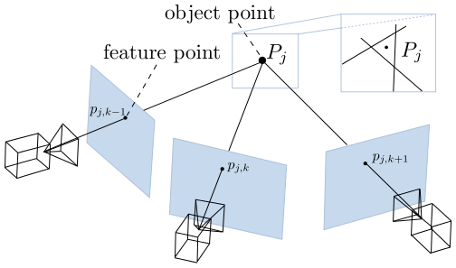
Multi view triangulation method. [9]

For multi-view triangulation, one solution can be to find such an X in 3D space which has a minimum sum of square distance with the 3D points lying on the bearing vector. Analytical solution for X can be found by taking the derivative of the loss function with respect to the 3D point and finding the 3D point where is the derivative of loss function equals zero. Assuming the $C_i$ is camera center of $i^{th}$ camera, $P_i$ is the point on $i^{th}$ bearing vector, $\lambda_i$ scalar distance between $C_i$ and $P_i$, and X is being optimal 3D point as a triangulation result , the triangulation result can be formulated as below.

Learning based Two View Stereo Reconstruction

Simaese networks for stereo matching[15].

Zbontar et al. [15] have initially shown that depth information can be extracted from rectified image pairs by learning a similarity measure on relevant image patches. They train their CNN-based siamese network as a binary classification network with similar and irrelevant pairs of patches.

GC-Net - deep stereo regression architecture[7].

Kendall et al. [7] proposed the network where they use 2D CNN with shared weights to retrieve rectified image pair features. In their work, they later used these feature maps to calculate a matching score-based cost volume, and as the last step, they use a 3D CNN-based autoencoder to regularize this volume.

Photogrammetry-based MVS

Patch-Based Multi-View Stereo [2] has proven being quite effective in practice. After an initial feature matching step aimed at constructing a sparse set of photoconsistent patches, in the sense of the previous section—that is, patches whose projections in the images where they are visible have similar brightness or color patterns—it divides the input images into small square cells a few pixels across, and attempts to reconstruct a patch in each one of them, using the cell connectivity to propose new patches, and visibility constraints to filter out incorrect ones. We assume throughout that n cameras with known intrinsic and extrinsic parameters observe a static scene, and respectively denote by $O_i$ and $I_i (i = 1, …, n)$ the optical centers of these cameras and the images they have recorded of the scene. The main elements of the PMVS model of multi-view stereo fusion and scene reconstruction are small rectangular patches, intended to be tangent to the observed surfaces, and a few of these patches’ key properties—namely, their geometry, which images they are visible in and whether they are photoconsistent with those, and some notion of connectivity inherited from image topology.

1. Matching Use feature matching to construct an initial set of patches, and optimize their parameters to make them maximally photoconsistent.
2. Repeat 3 times:
   • a) Expansion Iteratively construct new patches in empty spots near existing ones, using image connectivity and depth extrapolation to propose candidates, and optimizing their parameters as before to make them maximally photoconsistent.
   • b) Filtering Use again the image connectivity to remove patches identified as outliers because their depth is not consistent with a sufficient number of other nearby patches.

Learning-based MVS

State-of-the-art learning-based MVS approaches adapt the photogrammetry-based MVS algorithms by implementing them as a set of differentiable operations defined in the feature space. MVSNet [13] introduced good quality 3D reconstruction by regularizing the cost volume that was computed using differentiable homography on feature maps of the reference and source images.

Differentiable homography

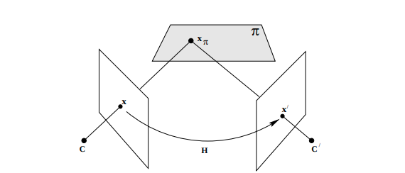
Two view homography [5] [4] [12]

Derivation with absolute pose

MVSNet overall architecture

MVSNet architecture [13]

MVSNet at first extract the deep features of the N (number of views) input images for dense matching. It applies convolutional filters to extract the feature towers scale.Each convolutional layer is followed by a batch-normalization (BN) layer and a rectified linear unit (ReLU) the last layer. Using features and the camera parameters, then we build cost volume regularization. We use differentiable homography for building this cost volumes.

The raw cost volume computed from image features are regularized later. Multi-scale 3DCNN have been used for cost volume regularization.This regularization step is designed for refining the above cost volume to generate a probability volume for depth inference.Depth that was regressed from probability volume is further refined using the 2DCNN network.

Bibliography

1. H. Aanæs, R. R. Jensen, G. Vogiatzis, E. Tola, and A. B. Dahl. Large-scale data for multiple-view stereopsis. International Journal of Computer Vision, pages 1–16, 2016.
2. Y. Furukawa and J. Ponce. Accurate, dense, and robust multi-view stereopsis. IEEE TPAMI, 32(8):1362–1376, 2010.
3. S. Galliani, K. Lasinger, and K. Schindler. Massively parallel multiview stereopsis by surface normal diffusion. June 2015.
4. D. Gallup, J. Frahm, P. Mordohai, Q. Yang, and M. Pollefeys. Real-time plane-sweeping stereo with multiple sweeping directions. In 2007 IEEE Conference on Computer Vision and Pattern Recognition, pages 1–8, 2007. doi: 10.1109/CVPR.2007.383245.
5. R. I. Hartley and A. Zisserman. Multiple View Geometry in Computer Vision. Cambridge University Press, ISBN: 0521540518, second edition, 2004.
6. H. Hirschmuller. Stereo processing by semiglobal matching and mutual information. IEEE Transactions on pattern analysis and machine intelligence, 30(2):328–341, 2007.
7. A. Kendall, H. Martirosyan, S. Dasgupta, P. Henry, R. Kennedy, A. Bachrach, and A. Bry. End-to-end learning of geometry and context for deep stereo regression. In Proceedings of the IEEE International Conference on Computer Vision, pages 66–75, 2017.
8. A. Knapitsch, J. Park, Q.-Y. Zhou, and V. Koltun. Tanks and temples: Benchmarking large-scale scene reconstruction. ACM Transactions on Graphics, 36(4), 2017.
9. P. Moulon, P. Monasse, R. Perrot, and R. Marlet. OpenMVG: Open multiple view geometry. In International Workshop on Reproducible Research in Pattern Recognition, pages 60–74. Springer, 2016.
10. J. L. Schönberger, E. Zheng, M. Pollefeys, and J.-M. Frahm. Pixelwise view selection for unstructured multi-view stereo. In European Conference on Computer Vision (ECCV), 2016.
11. F. Wang, S. Galliani, C. Vogel, P. Speciale, and M. Pollefeys. Patchmatchnet: Learned multi-view patchmatch stereo, 2021.
12. Wikipedia. Homography (computer vision). Wikipedia, 2013.
13. Y. Yao, Z. Luo, S. Li, T. Fang, and L. Quan. Mvsnet: Depth inference for unstructured multi-view stereo. European Conference on Computer Vision (ECCV), 2018.
14. Y. Yao, Z. Luo, S. Li, T. Shen, T. Fang, and L. Quan. Recurrent mvsnet for high-resolution multi-view stereo depth inference. Computer Vision and Pattern Recognition (CVPR), 2019.
15. J. Zbontar, Y. LeCun, et al. Stereo matching by training a convolutional neural network to compare image patches. J. Mach. Learn. Res., 17(1):2287–2318, 2016.