Gentle Introduction to SIREN

11 minute read

Published: October 10, 2022

We are interested in a class of functions $\Phi$ that satisfy equations of the form \begin{equation} F \left ( \mathbf{x}, \Phi, \nabla_\mathbf{x} \Phi, \nabla^2_\mathbf{x} \Phi, \ldots \right) = 0, \quad \Phi: \mathbf{x} \mapsto \Phi(\mathbf{x}). \label{eqn:functional} \end{equation}

Here we are going to discuss and focus on simple implementation of SIRENs which propose to leverage periodic activation functions for implicit neural representations. This work demonstrates that these networks, dubbed sinusoidal representation networks or SIRENs, are ideally suited for representing complex natural signals and their derivatives. While learning process, I went through following implementations (1,2,3) to understand better the SIRENs (and reuse the parts) and to come up to with simple testing implementation.

Authors also show that SIRENs can be leveraged to solve challenging boundary value problems, such as particular Eikonal equations (yielding signed distance functions), the Poisson equation, and the Helmholtz and wave equations. Lastly, we combine SIRENs with hypernetworks to learn priors over the space of SIREN functions.

Most of these recent network representations build on ReLU-based multilayer perceptrons (MLPs). While promising, these architectures lack the capacity to represent fine details in the underlying signals, and they typically do not represent the derivatives of a target signal well. This is partly due to the fact that ReLU networks are piecewise linear, their second derivative is zero everywhere, and they are thus incapable of modeling information contained in higher-order derivatives of natural signals. While alternative activations, such as tanh or softplus, are capable of representing higher-order derivatives, we demonstrate that their derivatives are often not well behaved and also fail to represent fine details.

The main highlights of this work are:

A continuous implicit neural representation using periodic activation functions that fits complicated signals, such as natural images and 3D shapes, and their derivatives robustly.
An initialization scheme for training these representations and validation that distributions of these representations can be learned using hypernetworks.
Wide range of applications: image, video, and audio representation; 3D shape reconstruction; solving first-order differential equations that aim at estimating a signal by supervising only with its gradients; and solving second-order differential equations.

Implementing SIRENs for images

A perceptron layer with periodic sine activations

SIREN propose a simple neural network architecture for implicit neural representations that uses the sine as a periodic activation function:

\[\begin{equation} \Phi \left( \mathbf{x} \right) = \mathbf{W}_n \left( \phi_{n-1} \circ \phi_{n-2} \circ \ldots \circ \phi_0 \right) \left( \mathbf{x} \right) + \mathbf{b}_n, \quad \mathbf{x}_i \mapsto \phi_i \left( \mathbf{x}_i \right) = \sin \left( \mathbf{W}_i \mathbf{x}_i + \mathbf{b}_i \right). \end{equation}\]

Here, $\phi_i: \mathbb{R}^{M_i} \mapsto \mathbb{R}^{N_i}$ is the $i^{th}$ layer of the network. It consists of the affine transform defined by the weight matrix $\mathbf{W}_i \in \mathbb{R}^{N_i \times M_i}$ and the biases $\mathbf{b}_i\in \mathbb{R}^{N_i}$ applied on the input $\mathbf{x}_i\in\mathbb{R}^{M_i}$, followed by the sine nonlinearity applied to each component of the resulting vector.

class SineLayer(nn.Module):

    def __init__(
            self,
            in_features,
            out_features,
            bias=True,
            first_layer=False,
            omega=30,
            custom_init=None,
    ):
        super().__init__()
        self.omega = omega
        self.linear = nn.Linear(in_features, out_features, bias=bias)

        if custom_init is None:
            paper_init(self.linear.weight, first_layer=first_layer, omega=omega)
        else:
            custom_init_function_(self.linear.weight)

    def forward(self, x):

        return torch.sin(self.omega * self.linear(x)) # sin(omega * (Wx + b))

Initialization scheme

The key idea in our initialization scheme is to preserve the distribution of activations through the network so that the final output at initialization does not depend on the number of layers. Note that building SINERs with not carefully chosen uniformly distributed weights yielded poor performance both in accuracy and in convergence speed.

Feel free to skip following paragraph for technical details.
Refer to paper and supplementary part for more mathematical and emprical insights.

Consider the output distribution of a single sine neuron with the uniformly distributed input $x \sim \mathcal{U}(-1, 1)$. The neuron’s output is $y = \sin(ax + b)$ with $a,b \in\mathbb{R}$. In supplementary part, paper shows that for any $a>\frac{\pi}{2}$, i.e. spanning at least half a period, the output of the sine is $y\sim\text{arcsine}(-1,1)$, a special case of a U-shaped Beta distribution and independent of the choice of $b$. Taking the linear combination of $n$ inputs $\mathbf{x}\in\mathbb{R}^n$ weighted by $\mathbf{w}\in\mathbb{R}^n$, its output is $y=\sin(\mathbf{w}^T\mathbf{x} + b)$. Assuming this neuron is in the second layer, each of its inputs is arcsine distributed. When each component of $\mathbf{w}$ is uniformly distributed such as $w_i \sim \mathcal{U}(-c/{\sqrt{n}}, c/{\sqrt{n}}), c\in\mathbb{R}$, author shows (see supplemental) that the dot product converges to the normal distribution $\mathbf{w}^T\mathbf{x} \sim \mathcal{N}(0, c^2/6)$ as $n$ grows. Feeding this normally distributed dot product through another sine is also arcsine distributed for any $c>\sqrt{6}$.

Paper proposes to draw weights with $c=6$ so that $w_i \sim \mathcal{U}(-\sqrt{6/n}, \sqrt{6/n})$. This ensures that the input to each sine activation is normal distributed with a standard deviation of $1$. Since only a few weights have a magnitude larger than $\pi$, the frequency throughout the sine network grows only slowly. Based on the experiments, authors suggest to initialize the first layer of the sine network with weights so that the sine function $\sin(\omega_0\cdot\mathbf{W}\mathbf{x} + \mathbf{b})$ spans multiple periods over $[-1,1]$. Experimental results shows $\omega_0=30$ to work well for all the applications in this work.

def paper_init(weight, first_layer=False, omega=1):

    in_features = weight.shape[1] # input shape

    with torch.no_grad():
        if first_layer:
            bound = 1 / in_features # first layer [-1/in_features, 1/in_features] uniform distribution
        else:
            bound = np.sqrt(6 / in_features) / omega # rest of the layers [-sqrt(6/in_features)/omega, sqrt(6/in_features)/omega] uniform distribution

        weight.uniform_(-bound, bound)

Multi Layer Sine Perceptrons for Grayscale Images

Consider the case of finding the function $\Phi:\mathbb{R}^2 \mapsto \mathbb{R}^1, \mathbf{x} \to \Phi(\mathbf{x})$ that parameterizes a given discrete intensity image $f$ in a continuous fashion. The image defines a dataset $\mathcal{D}=\{(\mathbf{x}_{i}, f(\mathbf{x}_i))\}_i$ of pixel coordinates $\mathbf{x}_i=(x_i,y_i)$ associated with their grayscale intensity $f(\mathbf{x}_i)$. The only constraint $\mathcal{C}$ enforces is that $\Phi$ shall output image intensity at pixel coordinates, solely depending on $\Phi$ (none of its derivatives) and $f(\mathbf{x}_i)$, with the form $\mathcal{C}(f(\mathbf{x}_i),\Phi(\mathbf{x}))=\Phi(\mathbf{x}_i) - f(\mathbf{x}_i)$ which can be translated into the loss $\tilde{\mathcal{L}} = \sum_{i} \vert \Phi(\mathbf{x}_i) - f(\mathbf{x}_i)\vert^2$.

Below you can see the experiment where only supervision on the image values holds, but also visualize the gradients $\nabla f$ and Laplacians $\Delta f$.

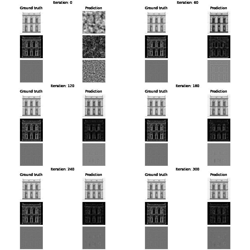
The code of the network is simple it takes inputs with two dimensional coordinate features and try to estimate one dimensional intensity value. Basically it is simple stacks of aforementioned Sine Layers.

class ImageSiren(nn.Module):

    def __init__(
            self,
            hidden_features,
            hidden_layers=1,
            first_omega=30,
            hidden_omega=30,
            custom_init=None,
            ):
        super().__init__()
        in_features = 2
        out_features = 1

        net = []
        net.append(
                SineLayer(
                    in_features,
                    hidden_features,
                    first_layer=True,
                    custom_init=custom_init,
                    omega=first_omega,
            )
        )

        for _ in range(hidden_layers):
            net.append(
                    SineLayer(
                        hidden_features,
                        hidden_features,
                        first_layer=False,
                        custom_init=custom_init,
                        omega=hidden_omega,
                )
            )

        final_linear = nn.Linear(hidden_features, out_features)
        if custom_init is None:
            paper_init(final_linear.weight, first_layer=False, omega=hidden_omega)
        else:
            custom_init(final_linear.weight)

        net.append(final_linear)
        self.net = nn.Sequential(*net)


    def forward(self, x):

        return self.net(x)

Image Dataset Loader:

The code samples below all image coordinates generate coordinates using np.meshgrid and np.stack. Scipy library was used to call Sobel and Laplace functions to get first and second order derivative of image.

For simplicity we are assuming that the image that we are trying to regress is a square image.

import numpy as np
from scipy.ndimage import laplace, sobel

def generate_coordinates(n):

    rows, cols = np.meshgrid(range(n), range(n), indexing="ij")
    coords_abs = np.stack([rows.ravel(), cols.ravel()], axis=-1)

    return coords_abs

class PixelDataset(Dataset):

    def __init__(self, img):
        if not (img.ndim == 2 and img.shape[0] == img.shape[1]):
            raise ValueError("Only 2D square images are supported.")

        self.img = img
        self.size = img.shape[0]
        self.coords_abs = generate_coordinates(self.size)
        self.grad = np.stack([sobel(img, axis=0), sobel(img, axis=1)], axis=-1)
        self.grad_norm = np.linalg.norm(self.grad, axis=-1)
        self.laplace = laplace(img)

    def __len__(self):
        return self.size ** 2

    def __getitem__(self, idx):
        coords_abs = self.coords_abs[idx]
        r, c = coords_abs

        coords = 2 * ((coords_abs / self.size) - 0.5)

        return {
            "coords": coords,
            "coords_abs": coords_abs,
            "intensity": self.img[r, c],
            "grad_norm": self.grad_norm[r, c],
            "grad": self.grad[r, c],
            "laplace": self.laplace[r, c],
        }

Using autograd for the network’s gradient and laplace calculation

torch.autograd.grad function was used to get gradient of function with respect to input coordinates. Laplacian similarly calculated using torch.autograd.grad by calculating divergence of the gradient.

class GradientUtils:
    @staticmethod
    def gradient(target, coords):
        return torch.autograd.grad(
            target, coords, grad_outputs=torch.ones_like(target), create_graph=True )[0]

    @staticmethod
    def divergence(grad, coords):
        div = 0.0
        for i in range(coords.shape[1]):
            div += torch.autograd.grad(
                grad[..., i], coords, torch.ones_like(grad[..., i]), create_graph=True,
            )[0][..., i : i + 1]
        return div

    @staticmethod
    def laplace(target, coords):
        grad = GradientUtils.gradient(target, coords)
        return GradientUtils.divergence(grad, coords)

Memorizing Grayscale image

Import functions

import matplotlib.pyplot as plt
import numpy as np
import torch
from torch.nn import Linear, ReLU, Sequential
from torch.utils.data import DataLoader
import tqdm
from dataset import PixelDataset
from net import GradientUtils, ImageSiren

Reading and standartization of a grayscale image

img_ = plt.imread("facade.png")
img = 2 * (img_ - 0.5) # standartization of data (-1,+1)
downsampling_factor = 8
img = img[::downsampling_factor, ::downsampling_factor] # reducing image resolution by skipping pixel rows and cols
size = img.shape[0]
dataset = PixelDataset(img)

Hyperparameters settings

We have two architectures to try out sirens and most prevalent mlp+relu architectures.

Here we have also multiple options to guide our loss function. You can optimize over intensity values, over gradient and laplacian values of the image.

n_epochs = 301
batch_size = int(size ** 2)
logging_freq = 20

model_name = "siren"  # "siren", "mlp_relu"
hidden_features = 256
hidden_layers = 3

target = "intensity"  # "intensity", "grad", "laplace"

Model Creation

Here we are creating our models, we choose adam as our optimizer.

if model_name == "siren":
    model = ImageSiren(
        hidden_features,
        hidden_layers=hidden_layers,
        hidden_omega=30,
    )
elif model_name == "mlp_relu":
    layers = [Linear(2, hidden_features), ReLU()]

    for _ in range(hidden_layers):
        layers.append(Linear(hidden_features, hidden_features))
        layers.append(ReLU())

    layers.append(Linear(hidden_features, 1))

    model = Sequential(*layers)

    for module in model.modules():
        if not isinstance(module, Linear):
            continue
        torch.nn.init.xavier_normal_(module.weight)
else:
    raise ValueError("Unsupported model")
    
dataloader = DataLoader(dataset, batch_size=batch_size)
optim = torch.optim.Adam(lr=1e-4, params=model.parameters())

Training process

Below you can see our training loop. As you see MSE were used as a loss criterion.

for e in range(n_epochs):
    losses = []
    for d_batch in tqdm.tqdm(dataloader):
        x_batch = d_batch["coords"].to(torch.float32)
        x_batch.requires_grad = True

        y_true_batch = d_batch["intensity"].to(torch.float32)
        y_true_batch = y_true_batch[:, None]

        y_pred_batch = model(x_batch)

        if target == "intensity":
            loss = ((y_true_batch - y_pred_batch) ** 2).mean()

        elif target == "grad":
            y_pred_g_batch = GradientUtils.gradient(y_pred_batch, x_batch)
            y_true_g_batch = d_batch["grad"].to(torch.float32)
            loss = ((y_true_g_batch - y_pred_g_batch) ** 2).mean()

        elif target == "laplace":
            y_pred_l_batch = GradientUtils.laplace(y_pred_batch, x_batch)
            y_true_l_batch = d_batch["laplace"].to(torch.float32)[:, None]
            loss = ((y_true_l_batch - y_pred_l_batch) ** 2).mean()

        else:
            raise ValueError("Unrecognized target")

        losses.append(loss.item())


        optim.zero_grad()
        loss.backward()
        optim.step()

    print(e, np.mean(losses))

    if e % logging_freq == 0:
        pred_img = np.zeros_like(img)
        pred_img_grad_norm = np.zeros_like(img)
        pred_img_laplace = np.zeros_like(img)

        orig_img = np.zeros_like(img)
        for d_batch in tqdm.tqdm(dataloader):
            coords = d_batch["coords"].to(torch.float32)
            coords.requires_grad = True
            coords_abs = d_batch["coords_abs"].numpy()

            pred = model(coords)
            pred_n = pred.detach().numpy().squeeze()
            pred_g = (
                GradientUtils.gradient(pred, coords)
                .norm(dim=-1)
                .detach()
                .numpy()
                .squeeze()
            )
            pred_l = GradientUtils.laplace(pred, coords).detach().numpy().squeeze()

            pred_img[coords_abs[:, 0], coords_abs[:, 1]] = pred_n
            pred_img_grad_norm[coords_abs[:, 0], coords_abs[:, 1]] = pred_g
            pred_img_laplace[coords_abs[:, 0], coords_abs[:, 1]] = pred_l

        fig, axs = plt.subplots(3, 2, constrained_layout=True)
        axs[0, 0].imshow(dataset.img, cmap="gray")
        axs[0, 1].imshow(pred_img, cmap="gray")

        axs[1, 0].imshow(dataset.grad_norm, cmap="gray")
        axs[1, 1].imshow(pred_img_grad_norm, cmap="gray")

        axs[2, 0].imshow(dataset.laplace, cmap="gray")
        axs[2, 1].imshow(pred_img_laplace, cmap="gray")

        for row in axs:
            for ax in row:
                ax.set_axis_off()

        fig.suptitle(f"Iteration: {e}")
        axs[0, 0].set_title("Ground truth")
        axs[0, 1].set_title("Prediction")

        plt.savefig(f"visualization/{e}.png")

Results

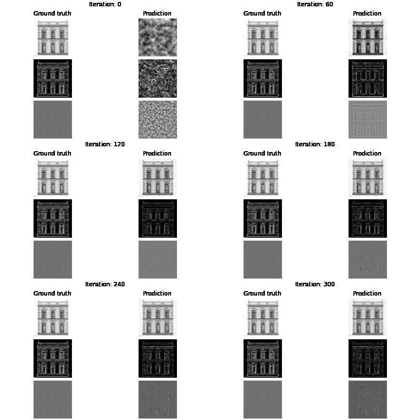
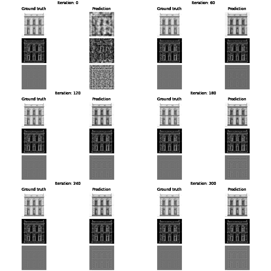
Below you can see the results based on different loss function guidance options

Intensity	Gradient	Laplace

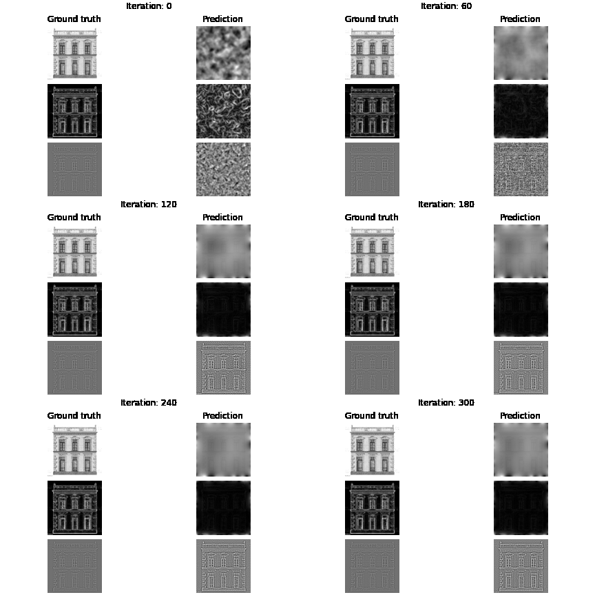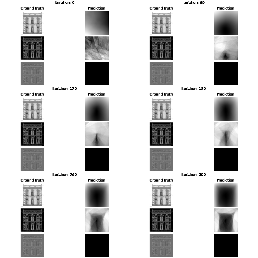
SIREN vs MLP+RELU trained on intensity values. As you may already see MLP may need more iterations to improve the intensity image, we also see that we have blank laplacian for MLP, since this type of architecture usually tends to reconstruct smooth data.

SIREN	MLP+RELU

You can get access to the source code using this github repo.

References

[1] Official SIREN project page
[2] lucidrain implementation
[3] Jan Krepl implementation

Share on

Twitter Facebook LinkedIn

Nail Ibrahimli