7 Incremental construction

One more method to the extrusion of Chapter 6, incremental construction exploits the property that an \(n\)-cell can be defined based on a set of \((n-1)\)-cells known to form its complete (closed) boundary. In practice, defining an \(n\)-cell in this manner is significantly more complex than doing so based on extrusion. However, unlike extrusion it permits the creation of cells of an arbitrary shape. It can also be applied cell by cell in increasing dimension, starting with the construction of isolated 0-cells (embedded in \(\mathbb{R}^n\)) first, and then constructing 2-cells, 3-cells and further based on their boundary, allowing for the incremental construction of objects of any dimension—hence the name given here.

This chapter describes an operation that permits the aforementioned process to be easily applied in practice using a topological data structure. Based on combinatorial maps (§4.3.6) and their fundamental operations (§5.1.1), it connects the separate boundary \((n-1)\)-cells together by computing the appropriate adjacency relationships between them, encapsulating low-level details such as the creation of new individual combinatorial elements and setting the correct orientation for the existing ones.

The chapter begins with some background on the operations and a description of the overall approach in §7.1. It then explains the steps needed to create the cells of each dimension in §7.2. §7.3 describes how the approach was implemented based on the Computational Geometry Algorithms Library (CGAL). §7.4 summarises some experiments based on this implementation, generating relatively large objects in up to 4D. Finally, §7.5 concludes the chapter with the possibilities to use incremental construction to build higher-dimensional datasets.

Most of this chapter is based on the paper:

@incollection{14icaa,
	address = {Kolkata, India},
	author = {Ken {Arroyo Ohori} and Guillaume Damiand and Hugo Ledoux},
	booktitle = {Applied Algorithms. First International Conference, ICAA 2014, Kolkata, India, January 13-15, 2014. Proceedings},
	editor = {Prosenjit Gupta and Christos Zaroliagis},
	month = {jan},
	note = {ISBN: 978--3--319--04125--4 (Print) 978--3--319--04126--1 (Online) ISSN: 0302--9743 (Print) 1611--3349 (Online)},
	pages = {37--48},
	publisher = {Springer International Publishing Switzerland},
	series = {Lecture Notes in Computer Science},
	title = {Constructing an n-dimensional cell complex from a soup of (n-1)-dimensional faces},
	volume = {8321},
	year = {2014}
}

7.1 Background and overall approach

Based on the Jordan-Brouwer separation theorem [Lebesgue, 1911; Brouwer, 1911], it is known that a subset of space homeomorphic to an \((n-1)\)-dimensional sphere¹⁰⁹ \(S^{n-1}\) in the \(n\)-dimensional Euclidean space \(\mathbb{R}^n\) divides the space into two connected components: the interior, which is the region bounded by the sphere, and the exterior, which is the unbounded region in which the sphere is a hole. This means that the principles of boundary representation as described in §3.1.2 extend to higher dimensions, and so an \(n\)-cell in a cell complex can be described (and therefore constructed) based a set of \((n-1)\)-cells that are known to form its complete (closed) boundary¹¹⁰.

The incremental construction method proposed in this chapter exploits this property by applying this process cell by cell in increasing dimension. Isolated vertices are first constructed, which are embedded in \(\mathbb{R}^n\) and are uniquely defined based on their coordinates. These vertices can then be connected to form individual edges, or instead to directly form cycles of implicit edges representing faces, as in most of the typical GIS approaches described in §3.2.2. Sets of faces can be connected to form volumes, sets of volumes to form 4-cells and so on.

In a similar manner as extrusion, presented in Chapter 6, this incremental construction process significantly reduces the conceptual complexity of defining and creating higher-dimensional objects. The \((n-1)\)-dimensional boundary of an \(n\)-cell is much easier to conceive than the original \(n\)-cell because it can be subdivided into multiple simpler \((n-1)\)-cells, which can be individually described and constructed using the same method.

However, applying this incremental construction process using a topological data structure is not that simple, as it involves many intricate small problems: finding the topological relationships between the cells, appropriately connecting them, keeping track of multiple connected components, avoiding the creation of duplicate cells (as part of the boundary of independently-described higher-dimensional cells), changing the orientation of cells on the fly (since those that have been created separately will often have incompatible orientations), and detecting non-manifold shapes (which would result in invalid structures), among others.

The incremental construction operator presented in this chapter solves all of the aforementioned issues efficiently. It is based on \(n\)-dimensional combinatorial maps with linear geometries and it is fully dimension-independent. As it generates all the incidence and adjacency relationships between \((n-1)\)-cells in an \(n\)-dimensional cell complex, it can also be used to obtain these relationships when needed, such as when multiple datasets are combined into one or when a non-topological representation is instead used (e.g. the Simple Features-like approach shown in §4.2.3).

In order to be efficient, the algorithm uses two basic techniques: (i) indexes on the lexicographically smallest vertex (§5.3) of certain cells, which are used in order to keep track of individual cells (which might be disconnected) and to access cells efficiently; and (ii) signature-generating traversals for specific cells [Gosselin et al., 2011], which are used to efficiently compare whether two cells are equivalent by checking if it is possible to find an isomorphism \(f\) that maps corresponding darts with equivalent (\(\beta\)) or reversed (\(\beta^{-1}\)) relations and which are embedded at the same location in \(\mathbb{R}^n\), as was shown in §5.5.

The incremental construction operation as described in this chapter is applicable only to perfect data. The \((n-1)\)-cells bounding an \(n\)-dimensional cell should thus form a manifold and perfectly match each other at their common \((n-2)\)-dimensional boundaries. However, the method can be easily extended to handle some more complex configurations, such as by cleaning the input data using the methods described in Chapter 10.

7.2 Incremental construction of primitives per dimension

The idea of the incremental construction algorithm is to construct cells individually, using lower-dimensional cells that have already been constructed in order to describe part of the boundary of a higher-dimensional cell. In terms of the darts of a combinatorial map, this sometimes implies the reuse of existing darts, and sometimes the creation of new ones which are connected to the existing ones. There is however no strict requirement that the cells are created in strictly increasing dimension, and so new cells can be easily added to an existing cell complex.

Due to the need to embed 0-cells into a point in space, as well as the oriented nature of a combinatorial map, the incremental construction method is different for 0-, 1- and 2-cells. 3-cells and those of higher dimensions follow a unified procedure. These cases are therefore described separately below, using as an example the creation of the pair of adjacent tetrahedra shown in Figure 7.1.

7.2.1 Vertices (0-cells)

The aim of the process of 0-cell construction is to create an isolated dart and an associated point embedding structure for every 0-cell, while avoiding having duplicate embedding structures having the same point coordinates. By making point embeddings unique—as defined by their coordinates—, they can be used to compare 0-cells without checking an entire tuple of coordinates. Moreover, by maintaining an index of all point embeddings and links from every point embedding to a dart there, it is possible to use this index to access the combinatorial structure at that point. In this manner, it is possible to find either an already free dart that can be reused, or a non-free dart that is part of a larger combinatorial structure, which can be then copied and its copy used instead.

Thus, calling a function \(\texttt{make_0_cell(}x_0, \ldots, x_n\texttt{)}\) with the coordinates \(x_0, \ldots, x_n\) describing an \(n\)-dimensional point, should use the index of 0-cells to return an existing dart embedded at that location (using an existing point embedding) if one exists, or a new dart embedded at that location (using a new point embedding) otherwise. In the latter case, the new point embedding and its associated dart should be added to the index. The result of calling this function for all the point coordinates of the vertices in Figure 7.1 is shown in Figure 7.2. Note that the result is identical whether the function is called once for every unique vertex, or multiple times (e.g. once for every vertex in every face or volume).

7.2.2 Edges (1-cells)

Generally, it is best to skip the generation of 1-cells and proceed directly to the creation of 2-cells from sequences of points. In order to represent an isolated edge in a combinatorial map not one but two darts are required: one embedded at each of the two vertices bounding the edge. More precisely, taking into account the (arbitrary) orientation defined for the edge, the dart embedded at the origin of the edge is connected to the destination by \(\beta_1\), and the destination is connected to the origin by \(\beta_1^{-1}\). Having two darts per edge is not a major problem, but it is wasteful as it often creates unnecessary darts and unnecessary connections between them that would later be deleted. For instance, if a single face that uses all the edges is created from its bounding edges, half of the darts lose their original purpose (i.e. to store a connection to their otherwise unlinked point embeddings) and will be eliminated¹¹¹, which is accompanied with having to reset the \(\beta\) relationships pointing to them.

In addition, as shown in §3.2.2, polygons can be easily described as an ordered sequence of vertices connected by implicit line segments between each consecutive pair. Therefore, incrementally constructing \(1\)-cells often brings no efficiency gains or practical benefits, and so it is normally best to skip dimension one, constructing 2D facets from a sequence of 0D points, 3D volumes from their 2D faces, 4-cells from their 3-cell faces, and so on.

However, there is an exception to this rule, as isolated edges and polygonal lines sometimes do need to be explicitly represented. In these cases, it is possible to simply follow the process described for 2-cells below, omitting sewing the last dart of the line segment or polygonal line to the first dart (and vice versa), and appropriately using the 1-cells index to find if a given 1-cell already exists, or otherwise to index the newly created 1-cell or 1-cells (in the case of a polygonal line).

7.2.3 Faces (2-cells)

Starting from the unique 0-cells obtained from the procedure presented in §7.2.1, in order to create a 2-cell from a sequence of 0-cells, three general steps are needed:

1. The procedure first checks if the 2-cell that is being requested already exists¹¹². Just as in the creation of 0-cells, a 2-cell being requested might have already been created, either independently or as part of a 3-cell. This can be easily checked using the index of 2-cells with the lexicographically smallest vertex of the 0-cells being passed, and finding if from a dart starting at the lexicographically smallest vertex and following the \(\beta_1\) or \(\beta_1^{-1}\) relations, one passes through the same point embeddings as those passed to this construction method.

2. Each of these 0-cells might be a \(1\)-free dart \(d\) (i.e. \(\beta_1(d) = \emptyset\)) and thus have no dart linked to it by \(\beta_1\), i.e. \(\beta_1^{-1}(d) = \emptyset\) or \(\forall d^\prime \nexists \beta_1(d^\prime) = d\), or if \(\beta_1^{-1}\) is not stored, \(\nexists d^\prime \mid \beta_1(d^\prime) = d\), in which case it can be used directly, such as in Figure 7.3. It can also be a non \(1\)-free dart or one that has a dart linked by \(\beta_1\) to it, which means that it is used as part of a \(1\)-cell (and possibly other higher dimensional cells).

   The darts that are already used as part of \(1\)-cells are more difficult to handle, as they can be reused only when the 1-cell they are part of is also part of the boundary of a geometrically identical \(2\)-cell as the one that will be constructed using this method. This needs to be tested in both possible orientations for the sequence of 0-cells, possibly resulting in the reversal of the orientation of some 1-cells. If a given dart cannot be reused (because it is part of a 1-cell that is not part of the 2-cell to be created), a copy of it has to be created. The result of this step is thus a list that contains for every 0-cell a reusable existing dart or a newly created dart.

3. The darts obtained in the previous step are 1-sewn sequentially (using \(\beta_1\) and \(\beta_1^{-1}\)), and the last is 1-sewn to the first, forming a closed cycle. During these sewing operations, the function checks whether every newly created edge (consisting of a pair of linked darts) is present in the index of 1-cells. If a given 1-cell is already there, the new edge’s dart is linked to its edge embedding structure. If a 1-cell is not there, the edge is added to the index¹¹³, a new edge embedding is created, and the edge’s dart is linked to it. Finally, the newly created 2-cell is then added to the index of 2-cells.

   In order to verify that the 2-cell being generated is a quasi-manifold, it is useful to assert that all darts that are \(1\)-free and have their \(\beta_1^{-1}\) relation set to \(\emptyset\) at the beginning of this third step, i.e. those that were not copied, should continue to be \(1\)-free and have a \(\beta_1^{-1}\) set to \(\emptyset\) until they are sewn. This condition, which is applied differently to the 1-cell, ensures that a vertex is not used twice within the same face, and as such, that the 2-cell is a quasi-manifold.

Figure 7.3 shows the incremental construction procedure for all the 2-cells of Figure 7.1, which consists of 7 2-cells and is thus obtained by 7 calls to the \(\texttt{make_2_cell}\) method.

(a)

(b)

(c)

(d)

(e)

(f)

(g)

(h)

7.2.4 Volumes (3-cells) and higher

The method to create \(i\)-cells from their \((i-1)\)-cell boundaries is identical for all \(i \geq 3\), allowing for a fully dimension-independent function to be created. This function consists of four general steps:

1. First of all, the procedure checks whether each \((i-1)\)-cell that is passed is \((i-1)\)-free or not. If it is \((i-1)\)-free, it is reused as part of the \(i\)-cell, such as in Figure 7.5. If it is not \((i-1)\)-free, then it is already part of a different \(i\)-cell, so a copy of it is made with a reversed orientation, as shown in Figure 7.6. This copy can then be used for the construction of the \(i\)-cell.

   For a given dart \(d\) that is known to be part of the \((i-1)\)-cell, this copy can be made by taking all the darts in the orbit \(C = \langle \beta_1, \ldots, \beta_{i-2} \rangle (d)\), creating a new set of darts \(C^\prime\), and inserting a new corresponding dart in \(C^\prime\) for every dart in \(C\). Using a function \(f : C \rightarrow C^\prime\) that maps a dart in \(C\) to its corresponding dart in \(C^\prime\), for every dart \(c \in C\) the \(\beta_1\) relations are set as \(\beta_1^{-1}\left(f\left(c\right)\right) = f\left(\beta_1\left(c\right)\right)\) and \(\beta_1\left(f\left(c\right)\right) = f\left(\beta_1^{-1}\left(c\right)\right)\). For the ones of higher dimensions, they are set such that \(\forall 2 \leq j \leq i-2\), \(\beta_j\left(f\left(c\right)\right) = f\left(\beta_j\left(c\right)\right)\).

   Note that the combinatorial structures are copied with reversed orientation, as this ensures that the two (old and new) can be directly \(i\)-sewn together, if necessary.

2. A temporary ridge index of the \(i\)-cell is built, containing all the \((i-2)\)-cells on the boundary of all \((i-1)\)-cells that have been passed to the construction method—not all the \((i-1)\)-cells in the cell complex—using their lexicographically smallest vertices, such that their index entries link to a usable dart in the \((i-2)\)-cell with a point embedding at the lexicographically smallest vertex. This dart should be one that is \((i-1)\)-free, either because it was already free as part of the combinatorial structure of the passed \((i-1)\)-cells, or because it is a copy (with reversed orientation) of one that was not \((i-1)\)-free.

3. Using the ridge index, \((i-1)\)-cells (i.e. facets) are \((i-1)\)-sewn along their common \((i-2)\)-cell boundaries (i.e. ridges). For this, for every \((i-2)\)-cell on the boundary of an \((i-1)\)-cell passed to the function, exactly one matching \((i-2)\)-cell should be found in the index, which should be equivalent as compared using the method described in §5.5 and might be of the same or opposite orientation (but should not be part of the same \((i-1)\)-cell or matched to itself). This criterion ensures that a quasi-\((i-1)\)-manifold will be constructed.

   If the two \((i-1)\)-cells are sewable along their common \((i-2)\)-cell boundaries, i.e. they have compatible orientations, they are directly sewn together. Otherwise, the orientation of the entire connected component of either of the two \((i-1)\)-cells should be reversed. If the two \((i-1)\)-cells have incompatible orientations but are part of the same connected component, the cell that is being requested is unorientable, and thus cannot be represented using combinatorial maps. Although not discussed further here, note that as long as it does forms a quasi-manifold it can however be represented using generalised maps.

4. Using the index of \(i\)-cells, the newly constructed \(i\)-cell is compared to others to check if it had already been created, which is also done using the lexicographically smallest vertex of the cell. If an equivalent \(i\)-cell (with the same or opposite orientation) is found, the function deletes the newly created darts of the cell and their corresponding index entries, and instead finally returns the existing \(i\)-cell. If an equivalent \(i\)-cell is not found, the newly created cell is added to the index and returned.

Figure 7.4 shows the incremental construction procedure for the two 3-cells of Figure 7.1.

7.3 Implementation and complexity analysis

The incremental construction algorithm has been implemented in C++11 and made available under the open source MIT licence at https://github.com/kenohori/lcc-tools. As the extrusion related code (§6.3), it requires and builds upon the CGAL packages Combinatorial Maps and Linear Cell Complex, among others.

For this prototype implementation, the lexicographically smallest vertex indices were implemented as C++ Standard Library maps¹¹⁴ for every dimension, using point embeddings as keys and lists of darts as values. Each dart in a list represents a separate cell (of the dimension of the index) that has that point as its lexicographically smallest. A custom comparison function is passed as a template so that the points are internally sorted in lexicographical order. As a map has \(O(\log n)\) search, insertion and deletion times and \(O(n)\) space [ISO, 2015, §23.4], all of these operations can be performed efficiently.

If a strictly incremental approach is followed, creating all \(i\)-cells before proceeding to the \((i+1)\)-cells, it is not necessary to maintain indices for all the cells of all dimensions at the same time. The only ones that are needed are those for: all \(i\)- and \((i-1)\)-cells, as well as a temporary index for the \((i-2)\)-cells on the boundary of the \((i-1)\)-cells for the \(i\)-cell that is currently being constructed. This means that only three indexes—one of which likely covers only a small part of the dataset—need to be kept at a given time.

Most of these indices can be easily built incrementally, adding new cells as they are created in \(O(\log c)\), with \(c\) the number of cells of that dimension, assuming that the smallest vertex and a dart embedded there are kept during its construction. The complexity of building any index of cells of any dimension is thus \(O(c \log c)\) and it uses \(O(c)\) space.

Checking whether a given cell already exists in the cell complex is more complex. Finding a list of cells that have a certain smallest vertex is done in \(O(\log c)\). In an unrealistically pathological case, all existing cells in the complex could have the same smallest vertex, leading to up to \(c\) quadratic time cell-to-cell comparisons just to find whether one cell exists. However, every dart is only part of a single cell of any given dimension¹¹⁵, so while every dart could conceivably be a starting point for the comparison, a single dart cannot be used as a starting point in more than one comparison, and thus a maximum of \(d_{\mathrm{complex}}\) identity comparisons will be made for all cells, with \(d_{\mathrm{complex}}\) being the total number of darts in the cell complex. From these \(d_{\mathrm{complex}}\) darts, two identity comparisons are started, one assuming that the two cells (new and existing) have the same orientation, and one assuming opposite orientations. Each of these involves a number of dart-to-dart comparisons in the canonical representations that cannot be higher than the number of darts in the smallest of the two cells. The number of darts in the existing cell is unknown, but starting from the number of darts in the newly created cell (\(d_{\mathrm{cell}}\)), it is safe to say that no more than \(d_{\mathrm{cell}}\) dart-to-dart comparisons will be made in each identity test, leading to a worst-case time complexity of \(O(d_{\mathrm{complex}} d_{\mathrm{cell}})\). Note that this is similar to an isomorphism test starting at every dart of the complex.

Finally, creating an \(i\)-cell from a set of \((i-1)\)-cells on its boundary is more expensive, since the \((i-2)\)-cell (ridge) index needs to be computed for every \((i-1)\)-cell. Following the same reasoning as above, it can be created in \(O(r \log r)\) with \(r\) the number of ridges in the \(i\)-cell, and uses \(O(r)\) space. Checking whether a single ridge has a corresponding match in the index is done in \(O(d_{\mathrm{cell}} d_{\mathrm{ridge}})\), with \(d_{\mathrm{cell}}\) the number of darts in the \(i\)-cell and \(d_{\mathrm{ridge}}\) the number of darts in the ridge to be tested. Since this is done for all the ridges in an \(n\)-cell, the total complexity of this step, which dominates the running time of the algorithm, is

\begin{equation*} \displaystyle\sum_{\mathrm{ridges}} O(d_{\mathrm{cell}} d_{\mathrm{ridge}}) = O(d_{\mathrm{cell}}^{2}). \end{equation*}

The analyses given above give an indication of the computational and space complexity of the incremental algorithm as a whole. However, it is worth noting that in realistic cases the algorithm fares far better than in these worst-case scenarios: the number of cells that have a certain smallest vertex is normally far lower than the total number of cells in the complex, most of their darts are not embedded at the smallest vertex, and from these darts most identity comparisons will fail long before reaching the end of their canonical representations.

Finally, one more nuance can affect the performance of this approach. When two connected components of darts with incompatible orientations have to be joined, the orientation of one of these has to be reversed. This is easily done by obtaining all the connected darts of one of the connected components, preferably the one that is expected to be smaller, and reversing their orientation 2-cell by 2-cell. Every dart \(d\) in a 2-cell is then \(1\)-sewn to the previous dart in the polygonal curve of the 2-cell (i.e. \(\beta_{1}^{-1}(d)\)). A group of \(n\) darts can thus have its orientation reversed in \(O(n)\) time. This is not a problem in practice since GIS datasets generally store nearby objects close together, but if a cell complex is incrementally constructed in the worst possible way, i.e. creating as many disconnected groups as possible, this could have to be repeated for every cell of every dimension, creating a very inefficient process.

7.4 Experiments

Simple comparisons with valid primitives

The CGAL Linear Cell Complex package provides functions to generate a series of primitives (line segments, triangles, quadrangles, tetrahedra and hexahedra) which are known to be created with correct geometry and topology, and can then be sewn together to generate more complex models. Models constructed in this manner were thus created independently and compared to those incrementally constructed using the method presented in this chapter. By using the approach shown in §5.5, it was possible to validate that they were equivalent.

A tesseract

In order to present an example in more than three dimensions, a tesseract was also incrementally constructed using the approach presented in this chapter, which is shown in Figure 7.5. A tesseract is a 4-cell bounded by 8 cubical 3-cells, each of which is bounded by 6 square 2-cells. It thus consists of one 4-cell, 8 3-cells, 24 2-cells, 32 1-cells and 16 0-cells.

Using the approach presented here, an empty 0-cell index is first created. Then, the 16 vertices of the tesseract, each vertex \(p_{i}\) being described by a tuple of coordinates \((x_{i},y_{i},z_{i},w_{i})\), were created as \(p_{i}=\texttt{make_0_cell(}x_{i},y_{i},z_{i},w_{i}\texttt{)}\), which returns a unique dart embedded at each location that is also added to the 0-cell index. At this point, the algorithm has built an unconnected cell complex consisting solely of 16 completely free darts.

An empty index of 2-cells is then created. Each of the tesseract’s 24 square facets are then built based on their vertices as \(f_{i}=\texttt{make_2_cell(}p_{j},p_{k},p_{l},p_{m}\texttt{)}\), which 1-sews (copies of) these darts in a loop and returns the dart embedded at the smallest vertex of the facet. These are added to the index of 2-cells. Since every vertex is used in 6 different 2-cells, each dart would be copied 5 times. The cell complex at this point thus consists of 24 disconnected groups of 4 darts each.

Next, an empty index of 3-cells is created and the index of 0-cells can be deleted. For each of the 8 cubical 3-cells, a function call of the form \(v_{i}=\texttt{make_3_cell(}f_{j},f_{k},f_{l},f_{m},f_{n},f_{o}\texttt{)}\) is made. At this point, an index of the 1D ridges of each face is built, which is used to find the 12 pairs of corresponding ridges that are then be 2-sewn together. When a 3-cell is created, it is added to the index. Since every face bounds two 3-cells, each dart is duplicated once again, resulting in a cell complex of 8 disconnected groups of 24 darts each.

Finally, the tesseract is created with the function \(t=\texttt{make_4_cell(}v_{1},v_{2},\dots,v_{8}\texttt{)}\). This can use the index of 2-cells to find the 24 corresponding pairs of facets that are then 3-sewn to generate the final cell complex.

The validity of this object was tested by checking whether it formed a valid combinatorial map, testing whether each cube was identical to a cube created with the Linear Cell Complex package, and manually verified the \(\beta\) links of its 192 darts.

2D+scale data

In order to test the incremental construction algorithm and its applicability to data incorporating non-spatial characteristics, a few 2D+scale datasets from Meijers [2011] using ATKIS data¹¹⁶, were also incrementally constructed. As shown in Figure 7.6, these datasets model the generalisation of a planar partition as a set of stacked prisms. Both of the simple datasets of this figure were created successfully in under a second.

A larger dataset, shown in Figure 7.7 and consisting of 698 polyhedra with a total of 457 185 faces, was used as a benchmark to test the performance of the algorithm. This dataset was processed without errors in roughly 30 minutes, including validation tests to ensure that every face created was a valid combinatorial map and that the faces of a volume formed a closed quasi-manifold.

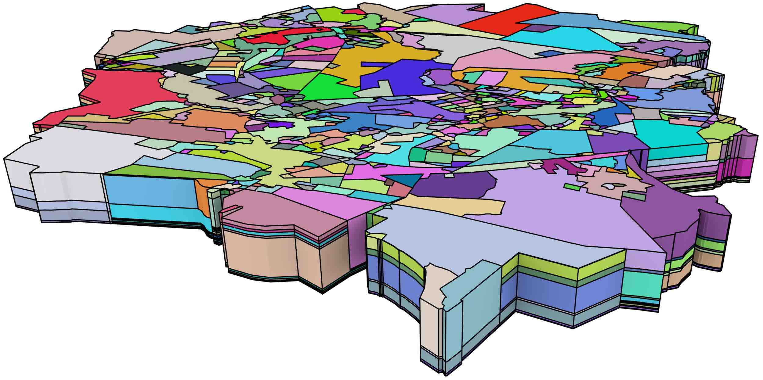
Figure 7.7: A large 2D+scale dataset from Meijers [2011], which uses equally spaced generalisation operations that merge two adjacent polygons.↩

In this latter dataset, an additional test was made using its first 250 polyhedra, which lie on the top of Figure 7.7, comparing the time used for the construction of vertices, faces and volumes with and without the use of indices. The results of both methods were equivalent using the approach shown in §5.5. On average, using indices resulted in a faster vertex construction time by a factor of 2 200, faster face construction by a factor of 56 and faster volume construction by a factor of 38. However, as Figure 7.8 shows, these speed gains are not uniform throughout the 250 polyhedra. The speed gained from using an index on the vertices increases roughly linearly on the number of constructed vertices, while that gained on from the faces index remains roughly constant between a factor of 50 and 60, and that gained from the volumes index tends to slowly increase as well.

(a)

(b)

(c)

Figure 7.8: Construction time speed-up from the use of indices on the (a) vertices, (b) faces and (c) volumes.↩

7.5 Conclusions

Creating computer representations of higher-dimensional objects can be complex. Common construction methods used in 3D, such as directly manipulating combinatorial primitives, or using primitive-level construction operations (e.g. Euler operators [Mäntylä, 1988]), rely on our intuition of 3D geometry, and thus do not work well in higher dimensions. It is therefore all too easy to create invalid objects, which then cannot be easily interpreted or fixed.

The incremental construction method proposed in this section follows a completely different approach, which has a solid underpinning in the Jordan-Brouwer separation theorem [Lebesgue, 1911; Brouwer, 1911]. By exploiting the principles of boundary representation, it constructs an \(i\)-cell based on a set of its bounding \((i-1)\)-cells. Since individual \((i-1)\)-cells are easier to describe than the \(i\)-cell, it thus subdivides a complex representation problem into a set of simpler, more intuitive ones. The method can moreover be incrementally applied to construct cell complexes of any dimension, starting from a set of vertices in \(\mathbb{R}^n\) as defined by a \(n\)-tuple of their coordinates, and continuing with cells of increasing dimension—optionally creating edges from vertices, then faces from vertices or edges, volumes from faces and so on.

While a set of \((i-1)\)-cells bounding an \(i\)-cell can be said to already form a complete representation of an \(i\)-cell, this is not sufficient for its representation in a topological data structure, which requires the topological relationships between the \((i-1)\)-cells to be computed. The incremental construction algorithm proposed in this section thus computes the relationships that are required for two data structures: generalised or combinatorial maps. However, these relationships are also applicable to most other data structures.

The algorithm is efficient due to its use of indices using the lexicographically smallest vertex of every cell per dimension, as well as an added index using the lexicographically smallest vertex of the bounding ridges of the cell that is being built. It generates an \(i\)-cell in \(O(d^{2})\) in the worst case, with \(d\) the total number of darts in the cell. However, it fares markedly better in real-world datasets, as cells do not generally share the same lexicographically smallest vertex. By checking all matching ridges within a cell’s facets, the algorithm can optionally verify that the cell being constructed forms a combinatorially valid quasi-manifold, avoiding the construction of invalid configurations.

A publicly available implementation of the algorithm has been made based on CGAL Combinatorial Maps, and its source code has been released under a permissive licence. It is worth noting that it is one of very few general-purpose object construction methods that has been described and implemented for four- or higher-dimensional cell complexes.

The implementation has been tested with simple 2D–4D objects, as well as with large 2D+scale datasets from Meijers [2011]. The constructed objects were tested to verify that they form valid combinatorial maps. The small objects were also manually inspected, visualised, and where possible, they were compared with equivalent objects known to be valid using the method discussed in §5.5.

While the incremental construction operation as described in this chapter works only with perfect data, small modifications could make it applicable to additional configurations. For instance, merging adjacent cells that can be perfectly described by a single cell with linear geometry (e.g. collinear edges and coplanar faces) as a preprocessing step can be used to handle cases where cells are subdivided only on one side of a boundary. Snapping points together can solve several common invalid configurations, such as those described in Chapter 10 and in Diakité et al. [2014].

Finally, the logical step forward at this point would be the use of the incremental construction algorithm for the creation of large higher-dimensional datasets. However, since to the best of my knowledge there are no large space-filling higher-dimensional datasets currently available—without even considering any validity criteria—, such tests could not be conducted within this thesis. The generation of such a higher-dimensional dataset is thus a necessary first step in this direction and is considered as a related piece of future work.

109. A generalisation of the concept of a sphere in arbitrary dimensions. A 0-sphere is the pair of points, a 1-sphere is a circle, and a 2-sphere a sphere. As opposed to disks and balls, circles and spheres are hollow.↩

110. This is true in practice. However, there are fractal-like pathological objects where this is not the case because their interior or exterior components are not homeomorphic to disks [Alexander, 1924]. While they do exist, this type of objects are certainly out of scope here.↩

(a)

(b)

Figure 7.1: (a) Two adjacent tetrahedra and (b) their representation as a combinatorial map.↩

Figure 7.2: Constructing the 0-cells of Figure 7.1 consists of creating exactly one dart embedded at each point. These darts are isolated (i.e. not linked by any \(\beta\) relations to the other darts). The direction of the arrows shown here is arbitrary.↩

111. These could be those embedded at the edges’ origin, destination or a mixture of the two.↩

112. This test can also be done at the end of the process, which makes it possible to use the easy cell comparison method described in §5.5. In that case, the newly created cells (in the form of darts) that are found to be redundant should be deleted and removed from (or not added to) the indices.↩

113. Here, depending on the kind of expected input data, it might be more convenient to index edges at their origin vertex rather than at their lexicographically smallest.↩

(a)

(b)

Figure 7.4: The construction of the 3-cells of Figure 7.1. (a) After \(\texttt{make_3_cell(}b,c,d,e\texttt{)}\). (b) Final result, after \(\texttt{make_3_cell(}e,f,g,h\texttt{)}\).↩

114. The exact implementation depends on the library that is used, but normally they are red-black trees.↩

115. This is true for the type of combinatorial maps with linear geometries that are handled here, but not necessarily so in the general case.↩

(a)

(b)

(c)

Figure 7.5: A tesseract as a combinatorial map: (a) the darts of its 7 inner cubes, (b) the darts of its 8 cubes, and (c) all of its darts shown together.↩

116. http://www.bkg.bund.de/nn_147094/SharedDocs/Download/Barrierefreie-Textversionen/EN-InfoMaterial/EN-Text-Vector-Data.html↩

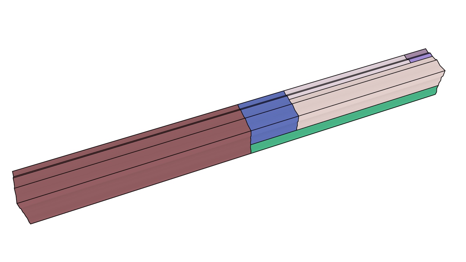
(a)

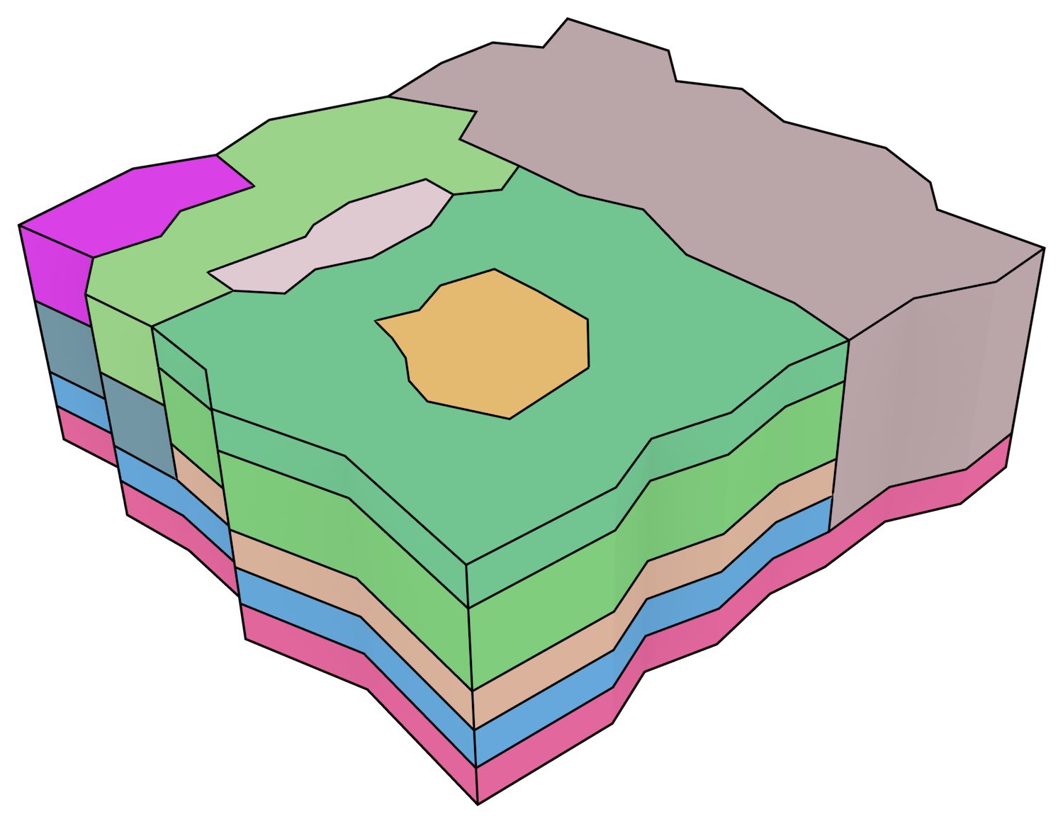
(b)

Figure 7.6: Simple 2D+scale datasets from Meijers [2011], which represent the generalisation of a planar partition by merging areas. The dataset shown in (a) has realistic scale intervals such that the generalisation operations are performed at scales that depend on the area of a polygon, while the dataset in (b) uses equally spaced generalisation operations.↩

6 Extrusion

Contents

8 Linking corresponding 3D models