Resit for the assignments

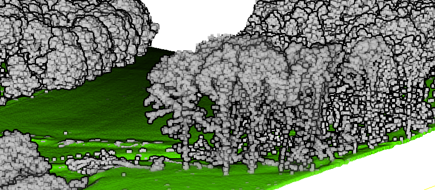
About point clouds, DTMs, and visualisation

Deadline is Friday 11 April 2025 at 8:59 (as the exam resit starts)

Late submission? 10% will be removed for each day that you are late.

This single assignment (with several steps) is the resit for the 3 assignments combined. It is worth 40% of the total mark of the course.

This is an individual assignment.

• Overview
• Step 0: Register for the resit to get the starting dataset
• Step 1: Download and prepare the dataset
• Step 2: DTM + nDSM creation (both gridded 50cmX50cm)
• Step 3: Compare your DTM with the official one from AHN4
• Step 4: Visualisation with iso-contours
• Marking
• What to submit and how to submit it

Overview

In this assignment you need to:

1. automatically classify a 300mX300m region of the AHN4 point cloud into ground and non-ground using the CSF algorithm
2. make a raster DTM using Laplace interpolation
3. make a raster nDSM with the method of your choice
4. compare your DTM rasters with the official AHN4 DTM raster
5. to help with visualisation you’ll have to implement a contouring algorithm

You have to use the following Python libraries (others are not accepted, or ask me first): numpy, startinpy, rasterio, scipy, laspy, fiona, shapely.

Step 0: Register for the resit to get the starting dataset

If you plan on doing this resit: send me an email (h.ledoux@tudelft.nl) and I’ll send you an AHN4 tile that you have to use. It’ll be a GeoTiles.

Step 1: Download and prepare the dataset

1. Download in LAZ format the AHN4 sub-tile you were assigned to: GeoTiles
2. Select a 300mX300m area in the tile that is most interesting (mix of buildings, terrains, forest, and some water), and provide its bounding box in the report
3. Extract the points from your region to the format you want for further processing

Step 2: DTM + nDSM creation (both gridded 50cmX50cm)

For this step, you need to write a Python program that performs all the steps automatically, and it should be useable for other areas in the Netherlands so the parameters should be exposed (see below).

You need to implement the Cloth Simulation Filter algorithm (CSF) as explained in the terrainbook.

Notice that you are not allowed to use the ground classification of AHN4 for this step! All the points should be use, and only the geometry is used to extract the ground.

You need to classify the points as ground and use those to generate the DTM with Laplace interpolation. You are not allowed to use startinpy’s interpolate() function, you need to implement it yourself (but you can use startinpy triangulation and other functions).

Your code should be a file called grid.py and it should have the following input parameters:

It should output 3 files in the same folder as grid.py:

1. a file called dtm.tiff representing the 50cm-resolution DTM of the area created with Laplace
2. a file called ndsm.tiff representing the 50cm-resolution nDSM of the area
3. the ground points in a file called ground.laz

For instance,

python grid.py mypc.laz 190000 303600 190100 303700 1.0 5.0 0.2

Use this in Python:

import argparse
parser = argparse.ArgumentParser()
parser.add_argument("ifile", help="input file in LAZ")
parser.add_argument("param1", help="param1 used for this and that")
parser.add_argument("param2", help="param2 used for this and that")
args = parser.parse_args()
print("ifile={}; param1={}; param2={})".format(ifile, param1, param2))

I will test your code with other areas/files.

Step 3: Compare your DTM with the official one from AHN4

How to compare them is left to you (you can use existing libraries and software), but highlight their differences and try to explain why they are different in the report.

For this step I don’t need the code, simply your analysis in the report.

Step 4: Visualisation with iso-contours

Implement the ideas described in “Conversion to isolines” in the terrainbook to produce a GeoPackage file of the contours lines at every meter (“full meters”, eg 1.0/2.0/3.0/etc).

Show me the results in the report and submit the code.

The Python code viz.py should also be submitted and have the following behaviour

and it should output a GeoPackage file called isocontours.gpkg where the lines have the elevation as an attribute.

You can create GeoPackage easily with “sister package” to rasterio called “fiona” (which uses the excellent “shapely”).

Marking

The following will be evaluated, each part refers to both the code (we will try to run it) and to the report (quality, completeness, analysis).

What to submit and how to submit it

You have to submit:

1. All the code you wrote with the names as defined above
2. a report (about ~20-25 pages) in PDF (no Word file please) where you elaborate on:
   • for each step, how did you perform it (in theory, I can read the code)
   • present the main issues you had and how you fixed them
   • give a reason why you picked certain parameters for the CSF algorithm
   • the differences between your results and the official DTM of AHN4
3. the DTM and the nDSM that you produced for the 250mX250m you chose

Those files need to be zipped and the name of the file is your studentID, for example 5015199.zip.

email me (h.ledoux@tudelft.nl) the ZIP before the deadline.

[last updated: 2025-02-06 11:07]